Speaker
Description
The effects of digital yield monitoring on greenhouse gas emissions in the US
Introduction
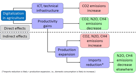
Digitalization in crop production likely affects the greenhouse gas (GHG) emissions from agriculture through several direct and indirect effects (Figure 1). Direct effects include more efficient use and therefore reductions of energy intensive inputs, such as fertiliser, plant protection, gasoline, and feed (D'Antonio et al., 2023). For example, GPS-led, self-driving tractors use less fuel (D'Antonio et al., 2023, Shockley et al., 2011, Jensen et al., 2012) and plant-specific input application requires less inputs (Finger et al., 2019, UNDP, 2021), and thus reduces emissions (Balafoutis et al., 2017). However, direct effects also include the initial set-up and energy use of digital infrastructure (García-Martín et al., 2019), which suggest an increasing effect of digitalization on emissions. Indirect effects result from cost reductions as a response to the direct effects because increasing levels of digitality lead quantities of other inputs to decrease. These cost reductions result in an increase in output quantity which can even cause a net increase of emissions (Brynjolfsson and McAfee, 2014, Paul et al., 2019). Apart from the level of digitalization in crop production, a second key determinant of GHG emissions in agricultural production is the output quantity.
Figure 1: Causal linkages between digitalization and GHG emissions.

Given that some of those effects work in opposite directions, this study determines empirically which set of effects dominates, relying on a panel dataset at the US state level between 1996 and 2010.
Methodology
To account for time-varying, unobserved heterogeneity, the analysis employs a Group Fixed Effects (GFE, Bonhomme and Manresa, 2015) approach to estimate the effects of digitalization and output quantity on GHG emissions from agriculture. Given that relations between emissions and both production (Bennetzen et al., 2015) and digitalization (Kopp et al., 2023) may be non-linear and to also allow for interacting effects, both the measure of digitality in crop production and production quantities enter as linear and as squared terms, as well as in the form of an interaction term. To avoid omitted variable bias while accounting for heterogeneity over time in the unobserved effects, we include time-varying, Group Fixed Effects (Bonhomme and Manresa, 2015) and control for income per capita. The econometric model is given by the following equation:

in which CCpc,s,c,t represents climate gas i ∈ {N2O, CH4, CO2}, emitted in state s at time t. prods,c,t stands for output quantity of crop c and digiymi,s,c,t is the share of the cultivated area of crop c on which digital yield monitoring technologies are employed. GDPpc,s,t stands for per capita income, and GFEg,t are the year-specific, fixed effects of groups of the state-crop-combination g. The β parameters represent coefficients to be estimated and εs,c,t captures normally-distributed, zero-centred errors.
Data
The unit of observation is state-crop-year. Those data stem from different federal agencies, including the U.S. Department of Agriculture (production quantities and spread of yield monitoring as a proxy for site specific fertilisation, pesticide application, etc.), the U.S. Environmental Protection Agency (methane and nitrous oxide emissions from production of specific crops), the U.S. Energy Information Administration (carbon dioxide emissions per state), and the U.S. Bureau of Economic Analysis (GDP per state). All numbers enter the estimation as per-capita values.
Results and discussion
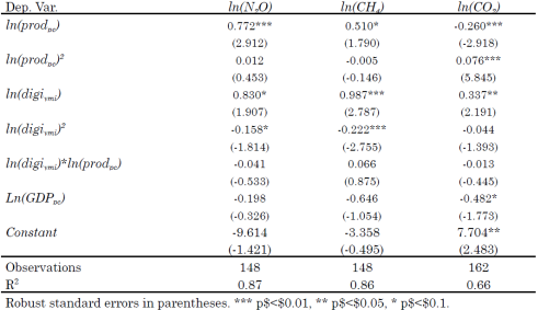
The estimation results are displayed in Table 1:
Table 1: Estimation results.

Given the quadratic relation between digitalization and emissions, the effects cannot be derived immediately by observing Table 1. We therefore differentiate the estimation equation with respect to the measure of digitalization and set it equal to zero to find the extremum of the respective parable. This procedure leads to the following extrema:
Table 2: Calculation of effects direction.

As the squared term is negative in the estimations of N2O and CH4, the respective functions are concave, indicating that the extreme values are maxima. For CO2, the squared term is statistically not significant, suggesting that the relation is linear. As for N2O and CH4, the maximum is below the median value of the measure for digitalization, the relation is decreasing at the sample median. For CO2, the linear effect is increasing.
Conclusions
The empirical analyses lead to the conclusion that for the case of methane and laughing gas, the productivity gains of digitalization in crop production reduce direct GHG emissions. In the case of carbon dioxide, the direct effects of the emissions generated through constructing and maintaining the digital infrastructure dominate over the reduced emissions from productivity gains.
References are not included in this abstract to save space.
